Fractals and Space-Filling Curves
Author: Aman Chaudhary
B.Sc. (H) Mathematics
Humans are fascinated by the beauty of nature, ranging from the Golden Ratio to the never ending nature of the Mandelbrot set (Fig 5.1), and the beauty it captures. An equally captivating idea is that of the Space-Filling Curves and Fractals. Mathematically speaking, A Space-Filling Curve is a curve whose range contains the entire 2-dimensional unit square. In simple terms, a curve that is capable of filling a given particular area (like a square grid), i.e. it passes through all the points that lie in that given space. It does seem quite fantastic when we find out that this continuous curve possesses infinite perimeter but doesn’t occupy infinite area.
It all started in 1878, when the mathematician G. Cantor had the novel idea of establishing a relation between R (1 Dimensional Space) and an n-dimensional space Rn. The aim was to somehow develop a surjective mapping from R to R2, which could include all the points in the plane, and such curves, as the name suggests, were called the Space-Filling Curves. Not going into the details of the topological space, we can think of Space-Filling Curve as a pattern shown in Fig 5.2. This seemingly alien curve, present in a unit square grid, when rearranged and replaced by four similar curves, gives us a continuous curve which looks four times denser than the previous one. Also, this process when iterated an infinite number of times, gives rise to the attractive pieces better known as fractals. Simply saying, Fractals are self-similar, never-ending, infinitely repeating patterns that look roughly the same no matter how much we zoom in.
The first Space-Filling Curve was proposed by Peano in 1890, and later on, similar curves were given by Hilbert, Moore, Sierpinski and many more. There lies an intimately close relation between Space-Filling Curves and Fractals. Space-Filling Curves have patrons and regularities that are highly linked to the self similar property of fractals. Though, the reader may note that not all the Space- Filling Curves are exactly self-similar. The curve mentioned above is the famous Hilbert Curve. The perimeter they encapsulate grows at an exponential rate. Given below are some beautiful seeds (basic iterator of the Space-Filling Curves).
Let us now look into some more facts about the wondrous Space-Filling curves, using one of the most popular curves, The Van Koch Snowflake Curve.
Koch Snowflake or Koch Star
- Constructing the infinite Snowflake: Start with taking an equilateral triangle. Divide each side into three equal segments and impose an identical equilateral triangle onto the middle segment (each side is replaced by 4 sides after each iteration), repeating it infinite times, gives rise to the Koch Snowflake Curve, founded by Neils Fabian Helge Van Koch.
- Infinite Perimeter: Space-Filling Curves are said to have an infinite perimeter, because surely even in the snowflake case, each time the new figure posses 4 times as many line segments as the previous figure, with the length of each segment being one-third of the last one, i.e. the perimeter of the new one is 4/3 of the previous perimeter whenever a bump is added. So following this process of adding infinite bumps and multiplying a finite perimeter of the initial equilateral triangle by 4/3 an infinite number of times, we actually land up having an infinite perimeter of the resultant Koch Snowflake.
- Finite Area: It does seem quite outrageous that a curve having infinite length but the area it bounds is finite and computable. To get an intuition of the finite area, think of a hexagon or maybe a circle (having a finite area) that can encircle the whole Koch Snowflake (Fig 5.6), thereby having an area less than that of the hexagon. The exact area of the Snow Flake comes out to be 2p3/5 times the area of the initial equilateral triangle (An exercise for the readers. Hint: Infinite G.P. concept).
- Continuous but not differentiable: The Koch SnowFlake is continuous everywhere but differentiable nowhere. Proofs show that there doesn’t lie even a one-sided tangent line at any point on this curve.
The Van Koch Snowflake Curve is a Fractal. A Fractal is a subset of a Euclidean space for which the fractal dimension strictly exceeds the topological dimension. In Fractal Geometry, a Fractal Dimension is a ratio providing a statistical index of complexity comparing how the detail in a Fractal pattern changes with the scale at which it is measured. It does not need to be a whole number. The Koch Snowflake Curve is said to have a fractal dimension equal to log 4/ log 3 = 1.262. Fractal Dimension of Sierpinski triangle is 1.585. It does seem uncanny to have such real valued dimensions, but that’s how we mathematicians are like.
Cohen’s Invention
In 1988, Nathan Cohen, a radio astronomer, came up with an idea of Infinite fractal antenna, since his landlord won’t allow him to put an antenna on the rooftop. He used the Koch curve type of antenna instead of the normal antenna having limited area but capable of picking more signals and not just one. This idea was later on improvised when Menger Sponge, a fractal curve which is a 3D generalization of the 1D Cantor set and 2D Sierpinski carpet having infinite surface area but zero volume, was used in cell phones for the same.
Everything in this universe depicts some kind of a fractal (until you get to the atomic level of that item), like measuring the coastline of a country. Space-Filling Curves are widely used to solve combinatorial optimization problems in industrial contexts, making fractal antennas, computer science engineering, etc. Even chromatin is a fractal and keeps DNA from getting entangled. But above all is the property of the Space-Filling Curves that says, “Every point lying on the Space-Filling Curve (which is bound to happen), seems to approach a limiting point in the Space as our Space-Filling Curve seems to approach a limiting curve”. Continuous Space-Filling Curves with this property find one of its uses in Google maps, to introduce cache locality: When you move a little bit while viewing the map, you want to be moving only a little bit in the memory, which is after all arranged linearly. So the next time you use the Google Maps, applaud the idea and charm of these Curves.
Figure 5.1
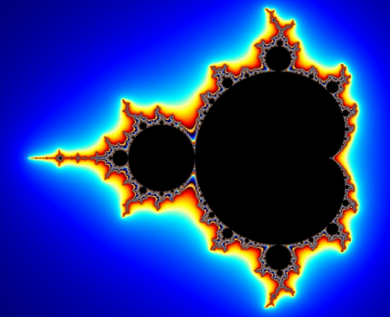
Figure 5.2


Figure 5.3
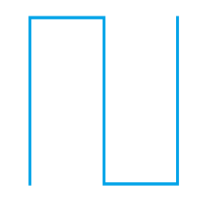
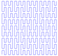
Figure 5.4
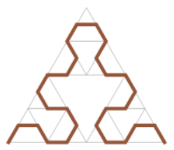
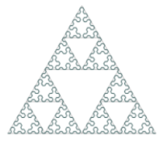
Figure 5.5
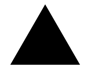
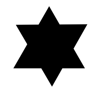
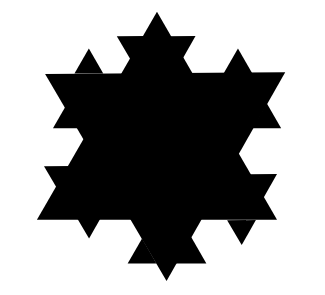
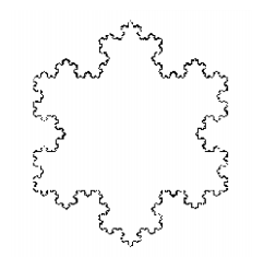
Figure 5.6
